Rubik's Cube Project Write-Up
Over the past few weeks, I’ve been working on a developing a program to assist the solution of a Rubik’s cube. The project started as an elaborate “joke,” after I messed up a friend’s Rubik’s cube and couldn’t put it back into its solved state. The goal of this project is to read in the state of an unsolved Rubik’s cube from a camera feed (or set of static images), and to provide step-by-step graphical instructions on how to solve the Rubik’s cube. Roughly, the project breaks down into four steps:
- Detect the squares on a Rubik’s cube’s face from a camera feed (or set of images).
- Determine what colors are on each square of each face of the cube.
- Solve the Rubik’s cube.
- Display solution steps to the user.
In this page, I’ll give a write-up of my current status on these four steps. The project isn’t yet complete, but I’m getting to a point where I want to move onto other things. In particular, some of the things that I will describe below haven’t yet been committed to the project’s git repository. However, the final result will likely end up being fairly similar.
1. Seeing the Cube
Since I have literally no background in computer vision, getting my computer to “see” the Rubik’s cube was easily the hardest part of this project - and it is something I still haven’t fully solved. For instance, my computer vision algorithm seems to go blind in dark low-contrast, settings, or (sometimes) when I present it with only red or blue squares. However, I’ve gotten my algorithm to a point where it’s successful at capturing the cube’s faces a decent fraction of the time. In the future, I may develop this a bit further… but at this point, I’m kind of tired of messing with it. So, I’ll most likely add some tools that allow the user to provide assistance if (when) the algorithm fails.
My cube detection algorithm was fairly heavily influenced by this write-up. However, the write-up (which is clearly a student’s project) is somewhat vague, and I was unable to get a working analogue of my own. To get everything working, I had to modify their algorithm a bit. For example, that author’s algorithm could successfully extract up to 3 faces from a single image, whereas my algorithm can only extract a single face at a time. In addition, my square detection algorithm requires some additional processing that is not described in that write-up.
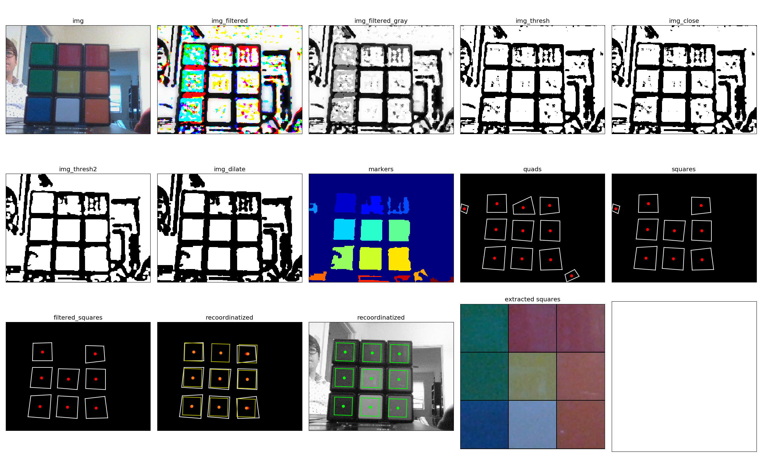
To detect a cube, I proceed as follows:
- Obtain a full RGB image with a single cube face.
- High-pass filter the image and convert the result to gray-scale.
- Threshold the high-pass filtered image.
- Apply a morphological closure to close up holes in the thresholded image.
- Clean the thresholded image by removing small clusters of noise pixels.
- Dilate the resulting image to thicken up the islands of black in the image.
- Split this image into contiguous regions (some of which will hopefully be squares!).
- Retain only the regions with quadrilateral convex hulls.
- Retain only the regions who’s boundaries are approximately square.
- Remove any squares that are too big or too small.
- Assuming we’ve observed at least one square in both the top/bottom row and both the left/right column, use this information to fill in missing squares.
- Extract the squares from the original RGB image.
The steps of the procedure look something like this:
2. Classifying the Squares’ Colors
Once the squares have been identified on each of the cube’s faces, we then need to identify what the squares’ colors are. For this purpose, I decided to use a simple classification algorithm, based on some very simple features extracted from each square. The features used in my algorithm are just the average RGB pixel value over the square, and pixel colors are classified using a support vector machine with a polynomial kernel fit.
To train the SVM classifier, I collected 24 sets of images for each of the 6 Rubik’s cube faces under various lighting conditions. Of these images, 17 were collected on my computer, and 7 were collected on my phone. The square detection algorithm was used to extract all 9 squares from each face. To facilitate easy labeling, I solved the cube prior to imaging it, and hence only needed to provide one color label per image. Features were generated by averaging the pixel colors over each image. In total, 1296 labeled training points were generated to feed into the classification algorithm.
The training data is plotted below, and demonstrates fairly robust class separation in the original feature space. Again, each data point represents the average pixel value collected over an extracted square. The data have been labeled according to their class color (as opposed to the RGB pixel value which they represent). Inspecting the graph, one can see that there is some small overlap between classes. In particular, the blue and white classes overlap a bit, which likely results from white squares reflecting blue light emitted from my computer’s monitor.
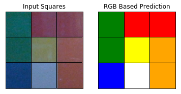
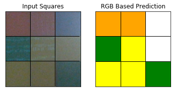
The following images demonstrate a successful classification result. The image on the left shows the set of squares extracted from this input image, and the image on the right shows the correctly predicted class labels for each square.
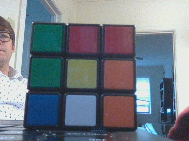
Unsurprisingly, the color classification algorithm isn’t perfect. It can get tripped up due to new lighting conditions that it hasn’t previously observed, images with significant noise, or bad lighting conditions. The following example shows a failed result based on this input image. The squares in the first and second row of the right-most column are both misidentified, most likely due to a combination of poor image quality and poor lighting conditions. The top-most square should be labeled blue (which is even a struggle for me to tell), but this square is incorrectly identified as white. The middle square should be labeled as yellow, however this square is misidentified as white. I’m not terribly concerned about the first error (since this one is hard), however it’s a bit surprising to me that the middle square was mislabeled, since the classification algorithm correctly identified the other similar looking yellow squares in the image.
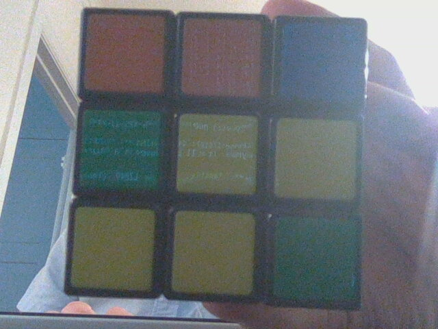
3. Solve the Cube
To solve the Rubik’s Cube, I mostly followed this method. I stayed pretty faithful to this procedure, although I did make a few minor modifications. Overall, this isn’t a very good solver, because it requires the cube to be in a very specific state in order to proceed. However, it’s pretty easy to understand, and hence it was pretty easy for me to implement.
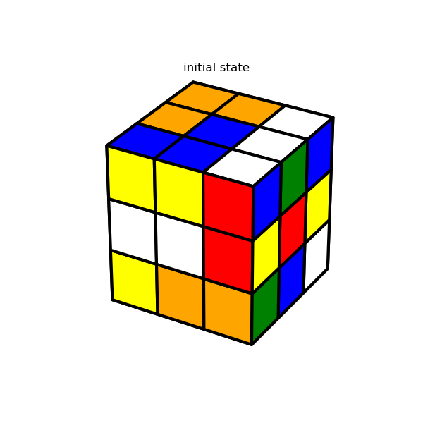
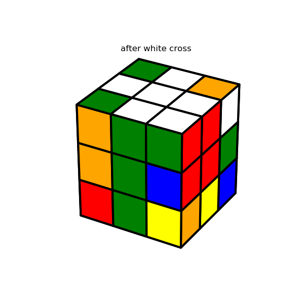
Since there’s not much interesting to say here, I’m just going to show a few images which demonstrate the solution algorithm’s major milestones. The interested reader can refer here for details.
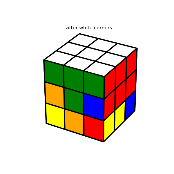
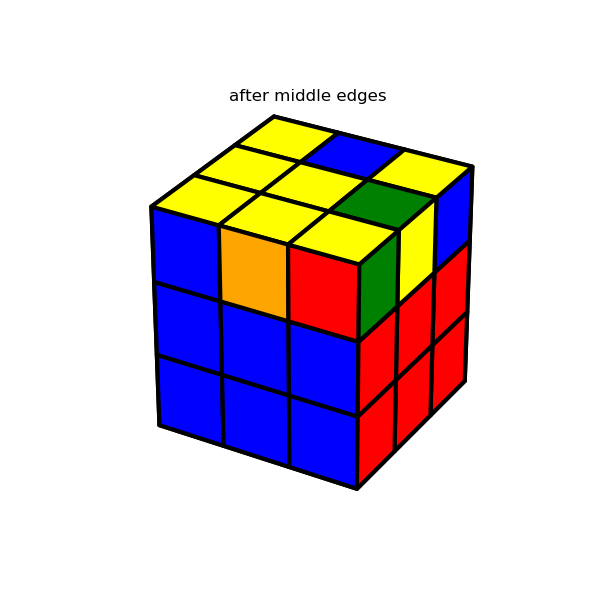
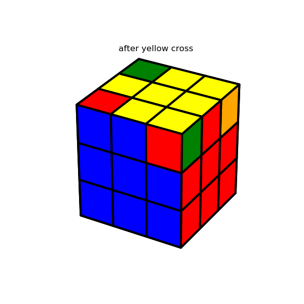
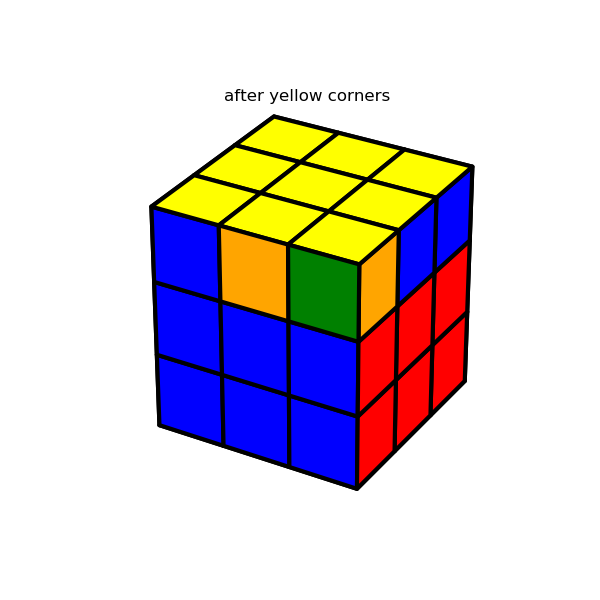
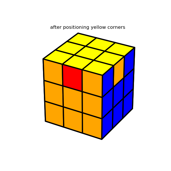
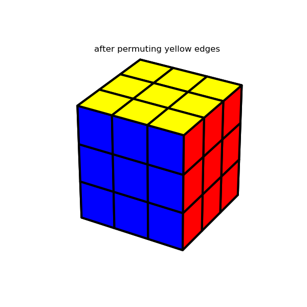
4. Display the results
As with the solver, there’s not much to say about the graphics, so I’ll just end with a random solution example. This example is actually a bit out of date, as it was generated before I had added in arrows to guide the user. One thing worth noting, is that the graphics are created using Matplotlib. This sort of thing isn’t really what Matplotlib was designed to do, but I kind of enjoyed shoe-horning in my use-case.