US State Hamiltonian Path Riddler
FiveThirtyEight’s Riddler problem for last week asked if it was possible to take a road trip in which you visit every continental US state without ever having to cross over the same border more than once - although returning to the same state is allowed. In this post, I’ll show that this in fact possible, and I’ll also provide a solution which only passes through each state exactly once.
The prompt problem can be viewed more abstractly as a question about identifying whether a Hamiltonian path exists on the continental US state border adjacency graph. Likewise, the question of whether it is possible to visit each state without returning to a state more than once can be recognized as a traveling salesman problem.
It turns out that you can pretty easily solve the prompt problem by hand (which I only realized after thinking quite a bit about the initial prompt), so I will begin by providing a hand-traced version that I was able to find. After that, I’ll discuss an optimal path that I found using simulated annealing. I should note though, if you print out a copy of the state border adjacency graph that I provide below, it wouldn’t be very hard to trace out an optimal path by hand.
One last thing: unlike in most of my other posts, the code to reproduce this post is not presented inline. Instead, the code to replicate this post can be found here.
Solution by Hand
Typically, I like to solve Riddler problems computationally with a view toward generalization, and in a manner which lends itself to interesting visualizations. However, it often happens that these puzzles can be easily solved by just picking up a pen and paper, which I ended up doing “first.”
In reality, “first” means that I only tried a by-hand solution after spending a bunch of time collecting shapefiles, adjacency graphs, setting up some rudimentary plotting tools, and reading about Hamiltonian paths and techniques to identify them. If I had actually traced out the solution by hand first, then I likely wouldn’t have bothered to make this post (:
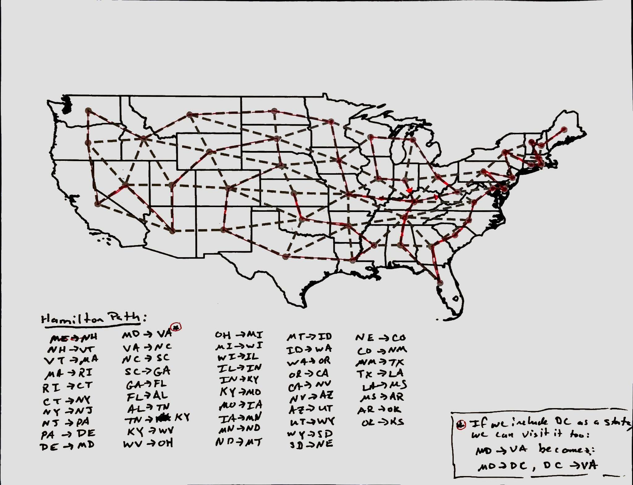
For the by-hand solution, I wasn’t actually concerned with minimizing the number of border crossings. I just started drawing from Maine (because Maine only has one border, a Hamiltonian path must necessarily begin or end there) and focused on finding a route which wouldn’t force me to use the same border crossing more than once. The Hamiltonian path that I found only required 48 distinct border crossings (I crossed into Kentucky twice), however, any path which visits all of the states must make at least 47 border crossings, so my by-hand solution was just one too many border crossings away from achieving the theoretical minimum.
The path for my by-hand solution was:
 ME NH VT MA RI CT NY NJ PA DE MD VA NC SC GA FL TN KY WY OH
 MI WI IL IN KY MD IA MN ND MT ID WA OR CA NV AZ UT WY SD NE
 CO NM TX LA MS AR OK KS
which looks as follows:
Optimal Solution Using Simulated Annealing
As indicated in the introduction, if we require that our road trip must only visit each state once, then we have turned the problem into a traveling salesman problem on the continental US state border adjacency graph. Although there are many ways to tackle this type of problem, I figured that I could make some interesting visualizations if I approached this problem using simulated annealing.
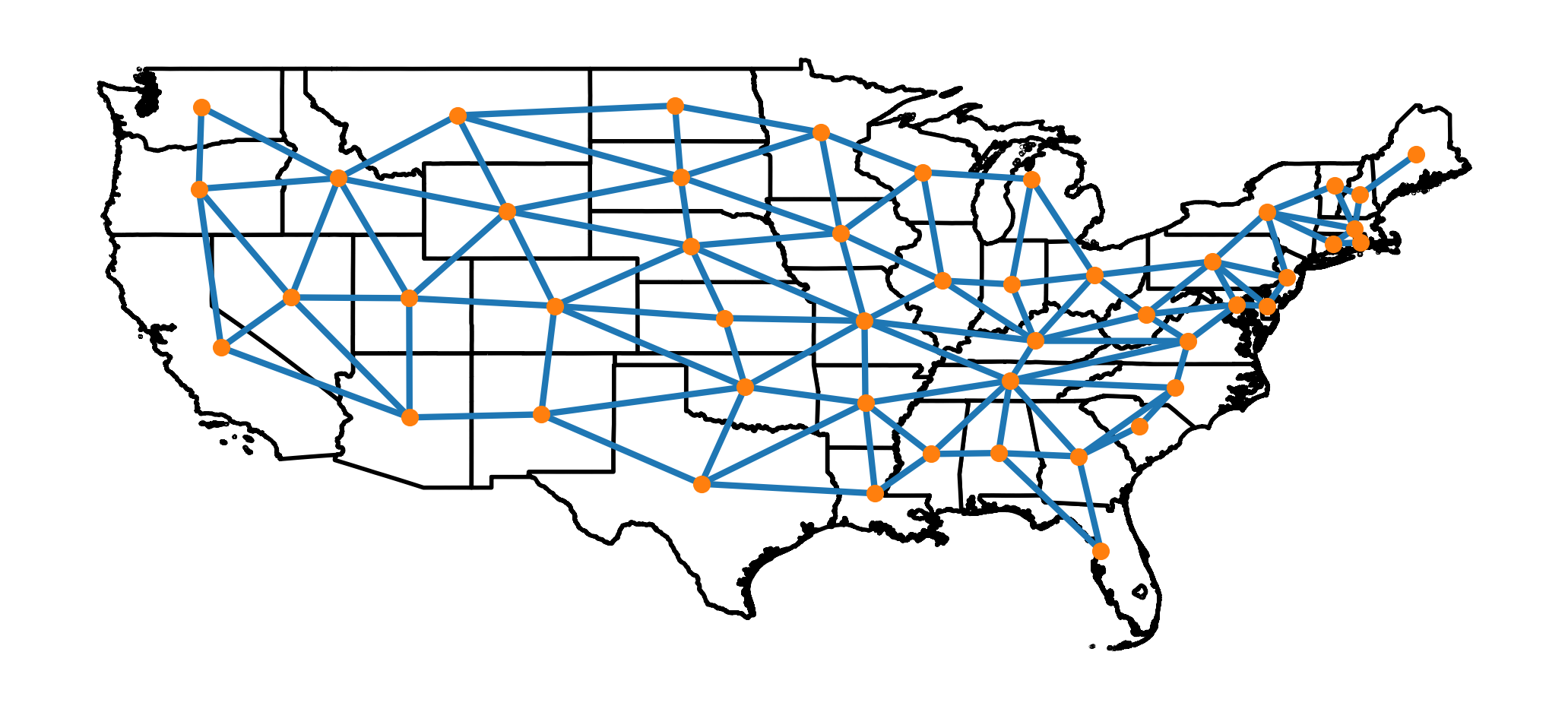
Adjacency graph
To set up the problem, I first obtained a list of the vertices for the US state border adjacency graph from here. (Note: the raw data includes DC, which must be removed for the current problem). In this graph, two states are considered adjacent if they share a border, and states that only meet in a corner are not considered to be adjacent to one another (e.g. CO and AZ are not considered to border one another).
The following image depicts the graph. In this plot, each state is represented by an orange node (plotted at the state’s centroid), and the graph’s vertices are represented by blue line segments connecting adjacent nodes.
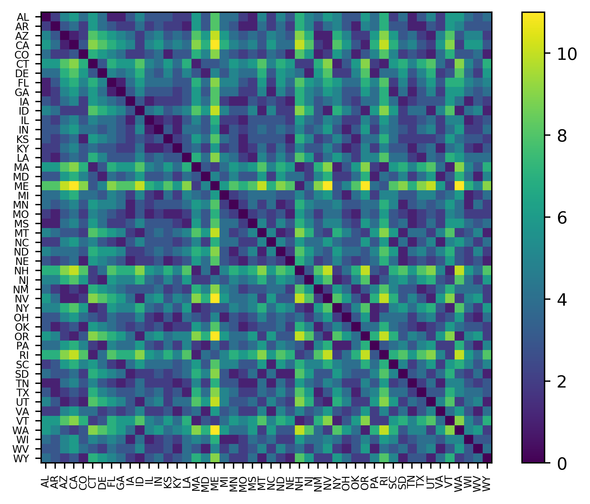
Graph distances
The next step in the solution was to compute the distances between states (so that I could compute the length of a path on the graph). Here “distance” means the distance in the sense of the adjacency graph, and does not refer to the physical distance between states. That is, for any pair of states, STATE_A and STATE_B, the distance between STATE_A and STATE_B is computed to be the minimum number of border crossings required to travel between them.
The following image shows the graph distance between all of the continental US states. In this image, the color of each square represents the distance between the states in that row and column. From this graph, we can see that states like Maine and California are very far apart from one another, with 11 border crossings required to travel between them.
Simulated annealing
Simulated
annealing is
based, in principle, upon the way that atoms settle into low energy
states as a material is slowly cooled. In this algorithm, the
objective to be minimized (in our case path_length) serves as an
analog to a system’s energy in material cooling. A temperature
parameter is introduced that is successively reduced as the algorithm
proceeds, which plays an analogous role to a real temperature when
slowly cooling a material. At each step, candidate solutions are
randomly generated that are near to the current candidate solution,
which mimics the process of atoms randomly jostling around in a
cooling material. The algorithm must then decide whether to adopt the
updated configuration or not. If a candidate reduces the objective, it
is always accepted. On the other hand, if a candidate increases the
objective, the algorithm will randomly decide whether to accept it in
a manner that depends upon the current temperature. Initially, when
the temperature parameter is high, the algorithm will have a
relatively high probability of adopting an inferior state, but as the
algorithm progresses and the temperature parameter is decreased, the
likelihood of accepting an inferior state is also reduced. This
property (of occasionally selecting worse configurations) allows the
procedure to randomly jump out of local minima and helps the algorithm
to trend toward a global minimum.
The simulated annealing algorithm that I used essentially follows the procedure outlined in Numerical Recipes in C, Chapter 10.9 to (approximately) solve the traveling salesman problem. The only real difference between that implementation and my implementation is that theirs requires the path to terminate at its starting point, while mine lets the path end at any node.
The simulated annealing implementation used here proceeds along the
steps shown in the following pseudo-code. In this pseudo-code, s
refers to a path on the graph, reverse(s, p1, p2) means to reverse
the path s between nodes p1 and p2, and transpose(s, p1, p2)
means to swap the nodes p1 and p2 on the path s.
    Let s = s_0
    Let T = T0

    ## Keep track of best paths identified
    best_path_length ← path_length(s)
    best_s_found ← s

    ## Only reduce temperature max_t_step times
    For t_step = 0 through max_t_step (exclusive):
        T ← (t_reduction_factor) * T

        ## Generate max_k candidates at each temperature T
	For k = 0 through max_k :

            ## select a neighboring path s_new by randomly generating
	    ## points and either reversing the path between them, or
	    ## transposing these points

	    randomly select distinct points, p1, p2 on the graph

	    If P(reverse) > random(0,1):
	        s_new ← reverse(s, p1, p2)
	    Else:
		s_new ← transpose(s, p1, p2)

            ## Decide whether to accept s_new or not

            If path_length(s_new) < best_path_length:
	        s ← s_new
  	        best_path_length ← path_length(s_new)
	        best_s_found ← s_new

            Else If P(path_length(s), path_length(s_new), T) ≥ random(0, 1):
	      	s ← s_new


    Output: best_s_found
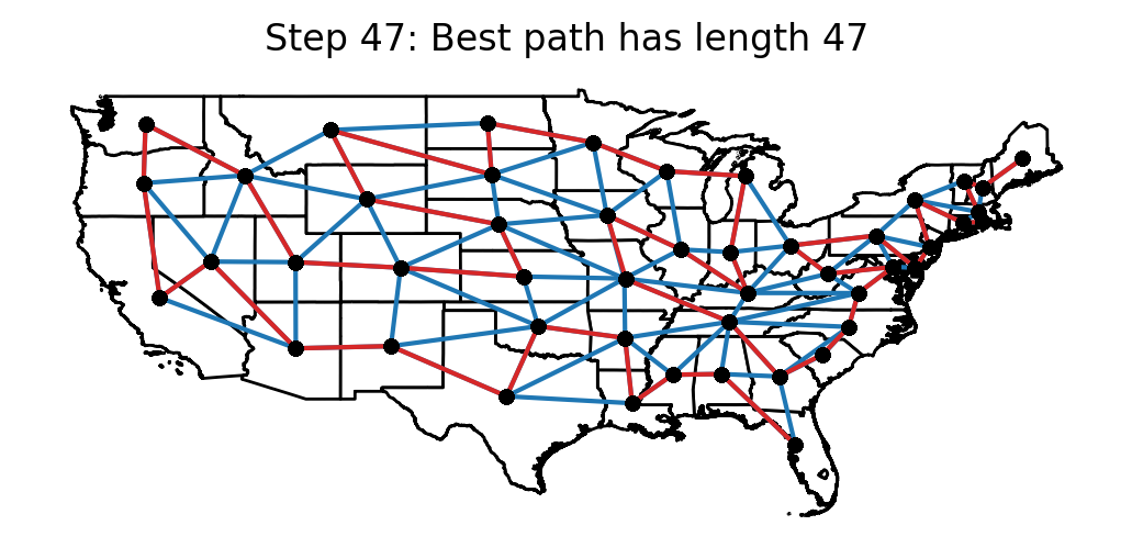
The following animation shows the candidate paths that were obtained after each temperature reduction in the algorithm. For each step, the best path length that the algorithm has seen up to that point is displayed.
Optimal solution
In the end, the optimal path that I found was:
 FL AL MS LA AR OK TX NM AZ NV CA OR WA ID UT CO KS NE WY MT
 SD ND MN WI MI IN KY IL IA MO TN GA SC NC VA MD WV OH PA DE
 NJ NY CT RI MA VT NH ME
which looks as follows: