Analyzing Error in Buffon's Needle Problem
A few months back, I began writing up a simple visualization in D3 to illustrate Buffon’s needle method for approximating \(\pi\) for a post celebrating Pi Day. The visualization took me a bit longer to complete than I had anticipated, so I ended up shelving the post at that time. However, while playing with the simulation, I noticed that the approximations to \(\pi\) from this method aren’t especially good. To quantify just how bad this approximation is, I worked out an asymptotic error analysis of this estimator. In this post, I have included my completed visualization along with the error analysis. For good measure, I also ran a Monte Carlo study of the error in Julia 🙂
Introduction
When I was a junior in high school, I was assigned do some sort of project about
\(\pi\) for Pi day. As you might be able to guess from the preceding sentence, I
can’t really remember what the assignment involved, but I do remember reading
Petr Beckman’s A History of Pi
for my presentation. This book describes the history of \(\pi\) and provides
several interesting methods that have been used in the past to estimate it.
One fun method discussed in this book is Buffon’s Needle
Problem, which is a
Monte Carlo method for estimating \(\pi\) that essentially boils down to
dropping needles over a regular grid and counting how many of them fall across
horizontal grid lines. With some time, graph paper, and needles, you could
simulate this process by hand. Since I didn’t have the patience for that, I
decided to quickly write up a visualization of the process,
which you can find below. The simulation requires a fairly
large number of needles in order to provide a decent estimation of \(\pi\), so
the results won’t be especially good - but you also won’t have to throw a lot of
needles by hand.
If you play around with the visualization a bit, you should begin to get a sense that this isn’t a very good way to estimate \(\pi\). Or, at least, I got that sense after clicking the button a lot of times while testing out the visualization. This got me thinking. The estimate was definitely bad, but how bad was it? To answer this obviously important question, I sat down and derived the behavior of the error estimate. The results can be found in this post, below the visualization (if you can’t wait, you can jump to it here). There, I derive a bound on the error which holds with a prescribed level of confidence.
Because I often like to validate my math, I decided that I’d run a simulation study to verify my error bound. I performed the simulation study in Julia, and have made the code and data available on github. Direct links are also provided below. If you’re just interested in how the simulation compares with the theoretical bounds, then you can jump directly to the results here.
Visualization
In Buffon’s needle problem, we drop spinning needles randomly in the plane and count the frequency of times that the needles fall across horizontal grid lines in order to obtain an estimate for \(\pi\). The following formula (which I’ll derive in the next section) is used:
\[\pi \approx 2 \cdot \frac{\text{needle length}}{\text{strip width between grid lines}} \cdot \frac{n_{\text{throws}}}{n_{\text{crossings}}}\]In the visualization below, grid lines are colored blue. Needles are colored red when they land across a grid line, otherwise they are colored gray.
Explaining Buffon’s Needle Problem
In this section I’ll give a brief overview of Buffon’s needle problem, and how it can be used to approximate \(\pi\).
As mentioned above, in Buffon’s needle problem, we drop spinning needles randomly in the plane and count the frequency of horizontal grid crossings in order to obtain an approximation for \(\pi\).
Let \(\ell\) denote the needle length and \(h\) the distance between horizontal strips. For simplicity (laziness), we’ll only consider the case where the needle length is smaller than the strip width (i.e. \(\ell \leq h\)). Since the strips are equally spaced and parallel to one another, we can focus our attention solely on how far away our needle lands from the nearest horizontal strip. Letting \(D\) denote the distance to the nearest strip, then \(D \sim \text{Uniform}[0, h/2]\). The needles will spin, landing with an angle \(\theta \sim \text{Uniform}[0, \pi)\) relative to the horizontal.
The next step is to compute the probability of a grid line crossing. The following diagram illustrates the situation:
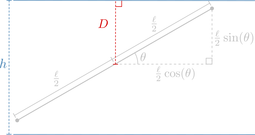
From the diagram, we can see that a crossing will occur just in case \(D < \frac{\ell}{2}\sin(\theta)\). Using this fact, and the fact that \(D\) and \(\theta\) are independent uniform random variables on \([0,h/2]\) and \([0,\pi)\) respectively, we see:
\[\begin{eqnarray} P(\text{crossing}) &=& \int_0^{\pi} \,d\theta \int_0^{\frac{\ell}{2} \sin(\theta)}\,dD \frac{1}{\pi} \frac{1}{h/2}\\ &=& \frac{2}{h\pi} \int_0^{\pi} \frac{\ell}{2} \sin(\theta) \,d\theta\\ &=& \frac{2\ell}{h\pi} \\ \end{eqnarray}\]For the remainder of the post, I will denote the crossing probability by \(p := P(\text{crossing})\).
Now, \(p\) can be estimated experimentally by simply counting how many times a needle falls across a horizontal grid line, \(\hat{p} = \frac{n_\text{crossings}}{ n_\text{throws}}\), plugging this into the expression above and re-arranging, we obtain our estimator for \(\pi\):
\[\boxed{\hat{\pi} = 2 \cdot \frac{\ell}{h} \cdot \frac{n_{\text{throws}}}{n_{\text{crossings}}}}\]Asymptotic Error Analysis
Now let’s investigate just how well \(\hat{\pi}\) estimates \(\pi\). Ultimately, we would like to answer a question like “how many needles do I need to throw in order to achieve some number of decimal digit accuracy in estimating \(\pi\) from \(\hat{\pi}\) “. Since \(\hat{\pi}\) is a random variable itself, our bounds will only hold with some given level of certainty - i.e. our error statement will involve \(\hat{\pi}\) falling within a confidence interval of \(\pi\).
To begin, note that \(n_\text{crossings} \sim \text{Binomial}(n_\text{throws}, p)\). As such, we have:
\[\begin{eqnarray} E[n_\text{crossings}] &=& p n_\text{throws}, \\ \text{Var}(n_\text{crossings}) &=& n_\text{throws}p(1-p).\\ \end{eqnarray}\]By the central limit theorem, if we define \(Z\) as:
\[\begin{eqnarray} Z &:=& \frac{n_\text{crossings} - p n_\text{throws}}{\sqrt{n_\text{throws} p(1-p)}}\\ &=& \sqrt{n_\text{throws}} \frac{\hat{p} - p}{\sqrt{p(1-p)}},\\ \end{eqnarray}\]then we have \(Z \rightarrow \text{Normal}(0, 1)\) as \(n_\text{throws} \rightarrow \infty.\)
Let \(\alpha \in [0, 1]\). The above discussion implies that when \(n_\text{throws}\) is large, we have that \(Z \in [-\Phi^{-1}(1 - \frac{\alpha}{2}), \Phi^{-1}(1 - \frac{\alpha}{2})]\) with probability \(P = 1 - \alpha\) (here \(\Phi^{-1}\) is the probit function). As such, the following inequality holds asymptotically with probability \(P\):
\[\left\vert\frac{\hat{p} - p}{\sqrt{p(1-p)}}\right\vert \leq \frac{1}{\sqrt{n_\text{throws}}}\Phi^{-1}\left(1 - \frac{\alpha}{2}\right).\]Re-arranging yields:
\[|\hat{p} - p| \leq \frac{\Phi^{-1}(1 - \frac{\alpha}{2})}{\sqrt{n_\text{throws}}} \sqrt{p(1-p)}.\]Using the fact that \(\pi = \frac{2\ell}{hp}\) and the analgous expression for \(\hat{\pi}\) in terms of \(\hat{p}\) and re-arranging a bit, we obtain:
\[\frac{2\ell}{h}\left|\frac{1}{\hat{\pi}} - \frac{1}{\pi}\right| \leq \frac{\Phi^{-1}(1 - \frac{\alpha}{2})}{\sqrt{n_\text{throws}}} \sqrt{\frac{2\ell}{h\pi}\left(1-\frac{2\ell}{h\pi}\right)}.\]Finally, after some manipulation (and using the approximation \(\hat{\pi} \approx \pi\) when \(n_\text{throws}\) is large), we get the following approximate error bound:
\[\boxed{\vert \hat{\pi} - \pi \vert \lessapprox \pi \sqrt{\frac{\pi}{2} - \frac{\ell}{h}} \cdot \Phi^{-1}\left(1 - \frac{\alpha}{2}\right)\cdot \sqrt{\frac{h}{\ell}} \cdot \frac{1}{\sqrt{n_\text{throws}}}.}\]Let’s pause for a moment to think about what this says. The inequality informs us that, regardless of how confident we want to be of our estimate (i.e. how close to \(0\) we take \(\alpha\)), and regardless of how we set up our experiment (i.e. how much smaller than \(h\) we take \(\ell\) to be), our estimate will converge like \(\mathcal{O}(\frac{1}{\sqrt{n_\text{throws}}})\). On the other hand, if we choose our needle size \(\ell\) to be small relative to our strip width \(h\) (i.e. if we make \(\frac{h}{\ell}\) big) then our bounding constant will be much larger – that is, we will pay a penalty in terms of guaranteeing accuracy if we don’t choose our needle length to be close to our strip width. Similarly, the more confident we want to be about our estimate, the more we have to pay in terms of our performance bound, since \(\Phi^{-1}(1 - \frac{\alpha}{2})\) increases as \(\alpha\) decreases.
Now, let’s use the above expression to determine how many throws are required to obtain a given level of accuracy. Letting \(\epsilon\) be the desired accuracy, the above expression gives:
\[\boxed{n_\text{throws} = \pi^2\left(\frac{\pi}{2} - \frac{\ell}{h}\right) \cdot \Phi^{-1}\left(1 - \frac{\alpha}{2}\right) ^2 \cdot \frac{h}{\ell} \cdot \frac{1}{\epsilon^2}.}\]Importantly, we see that the number of throws required to achieve an error of size \(\epsilon\) grows quadratically in \(1/\epsilon\). Hence, each additional decimal digit will require us to throw 100 times more needles! The following plot compares the number of throws required to achieve \(d = 1,2,\ldots,6\) decimal digit accuracy with 95% confidence when we use a horizontal strip width of one \(1.0\) units and needle lengths ranging from \(0.1,\ldots, 1.0\) units.

The chart demonstrates that using a needle length equal to our strip width (i.e. \(\ell=h\)) results in the smallest number of required throws to obtain a given number of correct decimal digits. In addition, the chart shows that we will need on the order of \(10^3\) throws in order to achieve a single decimal digit accuracy, around \(10^5\) for two, all the way up to \(10^{13}\) throws to get 6 digits correct. The following table summarizes the required number of throws for the optimal case where our needle length matches our strip width (\(\ell = h\)).
| Decimal Digits | Throws Required |
|---|---|
| 1 | 2164 |
| 2 | 216409 |
| 3 | 2.16409 * 10^7 |
| 4 | 2.16409 * 10^9 |
| 5 | 2.16409 * 10^11 |
| 6 | 2.16409 * 10^13 |
Simulation Study
Finally, I ran a simulation study to double check my error analysis. You can download the code to replicate the study directly here and I have also persisted the notebook for static viewing here.
In this study, I considered experimental set-ups with needles of length \(\ell = 0.1,0.2,\ldots,1.0\), a strip width of size \(h=1\), and a number of needles \(n_\text{throws}=10^2,10^3,\ldots,10^6\). I ran each experiment 1,000 times and computed the 95th percentile of my observed absolute error to compare against the 95% confident error bound derived above (i.e. the bound with \(\alpha=0.05\)). The following figure compares these two quantities across experimental set-ups. In this figure, the theoretical bounds are plotted as lines, while the observed data are plotted as circles.

The agreement is generally better with more data (which is unsurprising), but overall, the agreement with the theoretical results is pretty good. 🙂
Finally, since Buffon’s needle problem is interested in estimating \(\pi\) – and since I have mostly focused on the error in this method instead – I thought it might be fun to take a look at the the empirical distribution of \(\hat{\pi}\) for one of my experimental setups. The following figure shows how this distribution varies as a function of the number of needles thrown for the \(\ell = h\) case. The data are plotted using a dot-plot, while box-plots have been overlaid on top.

Summary statistics for this scenario are provided in the following table:
| Needles Thrown | Mean | Min | 25th Percentile | Median | 75th Percentile | Max |
|---|---|---|---|---|---|---|
| 100 | 3.1506 | 2.5641 | 2.9851 | 3.1250 | 3.2787 | 4.0000 |
| 1000 | 3.1433 | 2.9455 | 3.0912 | 3.1397 | 3.1898 | 3.4130 |
| 10000 | 3.1415 | 3.0623 | 3.1245 | 3.1422 | 3.1567 | 3.2196 |
| 100000 | 3.1415 | 3.1205 | 3.1364 | 3.1415 | 3.1465 | 3.1678 |
| 1000000 | 3.1417 | 3.1339 | 3.1400 | 3.1416 | 3.1434 | 3.1491 |