Infinite Chain Link Riddler
In this post, I will walk through my solution to the most recent Riddler problem. Here, we are asked to determine the path that is traced out by the tail end of a certain rigidly moving finite length chain with infinitely many links. While the behavior of each individual link in the chain is fairly complex, the path traced by its tail is surprisingly simple! (Although maybe this shouldn’t have been surprising! 🙂)
Introduction
This week’s Riddler asks us to consider a chain with infinitely many links. The links are ordered, and the first link has one end fixed at the origin while all other links are left free. The first link in the chain has length \(1\) and each successive link’s length decreases as a fixed proportion \(f \in (0, 1)\) of the preceding link (i.e if \(\ell_n\) is the length of the \(n^{th}\) link, then \(\ell_{n+1} = f \cdot \ell_n).\) This chain also has the property that, whenever you adjust the angle \(\theta\) between any pair of successive links, then every other sequential pair of links will bend so that it forms the same angle (i.e. \(\angle(\text{link}_n, \text{link}_{n+1}) = \theta\) for all \(n\)). The following figure illustrates the first few links of such a chain:
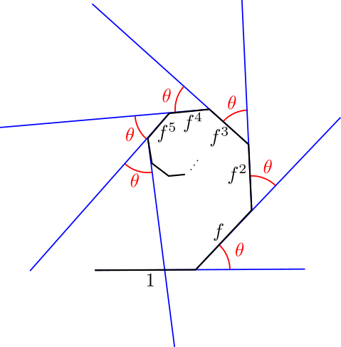
Since \(f < 1\), the chain has a finite length. Assuming that the chain starts out in a straight line (i.e. \(\theta = 0\)), we are asked: what curve does the chain’s tail end sweep out as we vary \(\theta\)?
In this post, I’ll show that the chain traces out a circle whose center and radius depend upon the scaling fraction \(f\).
Animation
Before we show that the chain’s free end traces out a circle, I thought it would be helpful to take a look at an animation of the problem. The following figure shows the behavior of a finite approximation to the chain as we vary \(\theta\):
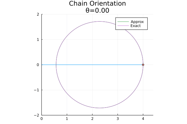
For this example, I took \(f = 0.75\), but the behavior shown here is representative of the general case. In the figure, I show the chain (in blue), an approximation to its tail (the orange dot), and the full path traced out by its tail (a finite approximation is shown in green, which is essentially indistinguishable from the exact solution shown in purple).
The animation was made interactively using Julia in a Pluto notebook. To run the code on your machine, you can download the notebook here. A static version can be found here, which can be executed interactively on binder.
Deriving an Expression for the Chain’s Tail
Let \(p_n\) denote the vertices along the chain. By assumption, the first vertex is constrained at the origin, so that \(p_0 = (0, 0)\). Since the lengths \(\ell_n\) of the chain’s links satisfiy the recurrence relation \(\ell_{n+1} = f\ell_n\) and \(\ell_0 = 1\), it follows that \(\ell_n = f^{n}\) for \(n=0,1,\ldots\) Next, let \(\Delta p_{n}\) denote the vector \(\Delta p_n = p_{n+1} - p_{n}\). Since each successive link is oriented at angle \(\theta\) relative to the previous link, and since the chain starts out parallel to the horizontal, the \(n^{th}\) link will be oriented at angle \(n \cdot \theta\) relative to the horizontal. From this, we see:
\[\Delta p_n(\theta) = f^{n} \cdot \left(\cos(n\theta),~\sin(n\theta)\right).\]Since \(p_0 = (0,0)\), the position of the \(n^{th}\) link is given by \(p_n = \sum_{k=0}^{\infty} \Delta p_k\). As such, the position of the chain’s tail is given by the infinite sum:
\[\gamma(\theta) = \sum_{n=0}^{\infty} \Delta p_n(\theta).\]Our goal will be to study how \(\gamma\) behaves as we vary \(\theta\).
In passing, I’ll note that the expressions for the coordinates of \(\gamma\) are respectively given by cosine and sine Fourier series. This fact didn’t really aid me in analyzing \(\gamma\) – but it probably explains how the problem’s author came up with the problem! That being said, because it’s often easier to work with complex Fourier series than to work with sine and cosine series, noticing that \(\gamma\) was described by a Fourier series prompted me to transition from thinking about the problem as a planar geometry problem, and to start thinking about it in terms of complex valued functions – which ultimately made the problem a lot easier! With this in mind, we now identify \((x,y) \leftrightarrow z = x+iy\) and proceed in polar form.
\[\begin{eqnarray} \Delta p_n &=& f^{n} \cdot \left(\cos(n\theta) + i \sin(n \theta)\right) \\ &=& f^{n} \cdot e^{in\theta}\\ \end{eqnarray}\]The series for \(\gamma\) is now very simple to compute:
\[\begin{eqnarray} \gamma(\theta) &=& \sum_{n = 0}^{\infty} \Delta p_n \\ &=& \sum_{n = 0}^{\infty} f^n e^{i\theta} \\ &=& \sum_{n = 0}^{\infty} (f e^{i\theta})^{n} \\ &=& \frac{1}{1 - f e^{i\theta}}\\ &=& \left(\frac{1 - f\cos(\theta)}{f^2 - 2f\cos(\theta) + 1}\right) + i \left(\frac{f\sin(\theta)}{f^2 - 2f\cos(\theta) + 1}\right) \end{eqnarray}\]Here, I have used the expression for the sum of a convergent geometric series on the fourth line, and on the last line, I have used WolframAlpha (since I was feeling lazy 🙂). This last formula is harder to work with than the formula on the second to last line, so we’ll mostly focus on the penultimate formula. On the other hand, the last formula does provide some useful insight, as well as being fairly useful for plotting.
Showing That the Image of \(\gamma\) is a Circle
Although it’s not immediately clear from the expressions above, the curve \(\gamma\) does in fact trace out a circular arc as we vary \(\theta\). To demonstrate this, it will suffice to show that all points on \(\gamma\) are equidistant from some central point/complex number \(c\). A candidate for \(c\) can be identified from the last expression for \(\gamma\) by looking at the average and extremal real-coordinate values on the interval \([0, \pi]\). To that end, notice that
\[\text{Real}\{\gamma\}(\theta) = \frac{1 - f\cos(\theta)}{f^2 - 2f\cos(\theta) + 1} = \frac{1}{1 + f\cos(\theta)}\]so the real part of \(\gamma\) is largest when \(\cos(\theta) = - 1\), for which \(\gamma = \frac{1}{1 - f}\), and smallest when \(\cos(\theta) = 1\), where \(\gamma = \frac{1}{1+f}\). The average of these extremal values is the real number \(c = \frac{1}{1 -f^2}\), which we now show is equidistant from all points on \(\gamma\):
\[\begin{eqnarray} \left| \gamma(\theta) - c\right| &=& \left|\frac{1}{1 - fe^{i\theta}} - \frac{1}{1 - f^2}\right| \\ &=&\left|\frac{fe^{i\theta} - f^2}{(1 - fe^{i\theta})(1 - f^2)}\right|\\ &=& \frac{|f||e^{i\theta} - f|}{|1 - fe^{i\theta}||1 - f^2|}\\ &=& \frac{|f||e^{i\theta} - f|}{|e^{-i\theta} - f||1 - f^2|}\\ &=& \frac{f}{1 - f^2}\\ \end{eqnarray}\]Since this is constant, we conclude that \(\gamma\) is constrained to live on a circle of radius \(\frac{f}{1-f^2}\) centered at \(z = \frac{1}{1-f^2}\). A little more thought allows us to conclude that \(\gamma\) visits every point on this circle, and in fact it is bijective onto this circle for \(\theta \in [0, 2\pi)\).
Alternate Approach
An alternative way to show that the image of \(\gamma\) is contained in a circle comes from complex function theory. To that end, note that (for \(f\neq0\)) the function \(z \mapsto \frac{1}{1 - fz}\) is a Möbius transformation of the complex plane. Since Möbius transformations preserve “generalized circles”, it follows that the image of the circle \(\theta \mapsto e^{i\theta}\) under \(\gamma\) is either a circle or a line. Since \(\gamma\) clearly isn’t a line (see that e.g., \(\gamma(\pi/2) = 0 + \frac{f}{f^2 + 1}\cdot i\) is not colinear with the real numbers \(\gamma(0) = \frac{1}{f^2-1}\) and \(\gamma(\pi) = \frac{1}{f^2+1}\)), we can conclude that the image of \(\gamma\) must be a circle.